2.2 - Linear Motion Graphs

Interpreting Graphs

Graph	Meaning
Displacement–time	Gradient gives velocity. A horizontal line indicates rest; a straight sloping line indicates uniform velocity; a curve with increasing gradient indicates increasing velocity.
Velocity–time	Gradient gives acceleration; area between the graph and time axis gives displacement with its direction. A horizontal line indicates uniform velocity; a straight sloping line indicates uniform acceleration.
Acceleration–time	A line on the time axis indicates zero acceleration; a horizontal line above it indicates uniform positive acceleration; an upward-sloping line indicates increasing acceleration.

v = \frac{Δ s}{Δ t}, a = \frac{Δ v}{Δ t}

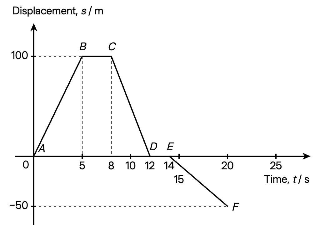
Taking motion to the right as positive, a motorcycle:

0–5 s: moves from $s = 0$ to $s = 100 m$ ; $v = (100 - 0) /5 = 20 m s^{- 1}$ .
5–8 s: stays at $s = 100 m$ ; $v = 0$ .
8–12 s: returns to $s = 0$ ; $v = (0 - 100) /4 = - 25 m s^{- 1}$ .
12–14 s: rests at the original point; $v = 0$ .
14–20 s: moves to $s = - 50 m$ ; $v = (- 50 - 0) /6 = - 8.33 m s^{- 1}$ .

Total distance $= 100 + 100 + 50 = 250 m$ ; total displacement $= 100 - 100 - 50 = - 50 m$ .

Average speed = \frac{250}{20} = 12.5 m s^{- 1}

Average velocity = \frac{- 50}{20} = - 2.5 m s^{- 1}

The negative velocities indicate motion to the left.

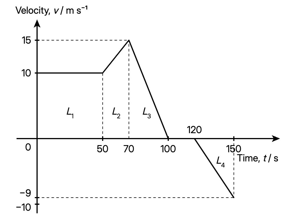
For a bicycle with motion to the right taken as positive:

0–50 s: $v = 10 m s^{- 1}$ ; $a = 0$ .
50–70 s: $v$ rises from 10 to 15 $m s^{- 1}$ ; $a = (15 - 10) /20 = 0.25 m s^{- 2}$ .
70–100 s: $v$ falls from 15 to 0; $a = (0 - 15) /30 = - 0.5 m s^{- 2}$ . The bicycle slows while moving right.
100–120 s: $v = 0$ ; the bicycle rests.
120–150 s: $v$ changes from 0 to $- 9 m s^{- 1}$ ; $a = - 9/30 = - 0.3 m s^{- 2}$ . Its speed increases as it moves left.
Areas above the time axis are 500 m, 250 m and 225 m; the area below has magnitude 135 m.
Distance is the sum of the area magnitudes: $500 + 250 + 225 + 135 = 1110 m$ .
Displacement uses signed areas: $500 + 250 + 225 - 135 = 840 m$ to the right.

Video analysis with Tracker can represent motion using displacement–time, velocity–time and acceleration–time graphs.
Convert displacement–time to velocity–time by finding each segment’s gradient. Convert velocity–time to acceleration–time in the same way.
Determine displacement from the area under a velocity–time graph; divide a complex area into rectangles, triangles or trapeziums.
Displacement example: displacement rises from 0 to 6 m in 0–6 s, stays at 6 m in 6–12 s, then rises to 10 m in 12–20 s. The corresponding velocities are 1, 0 and 0.5 $m s^{- 1}$ .
Kassim’s car: moves at 30 $m s^{- 1}$ for 6 s, then slows uniformly to rest at 10 s.
- Displacements: $(30) (6) = 180 m$ and $\frac{1}{2} (30) (4) = 60 m$ ; total 240 m.
- Accelerations: 0 and $(0 - 30) /4 = - 7.5 m s^{- 2}$ .
- Its displacement–time graph is initially straight, then curves with decreasing gradient to zero at 10 s.

Hasri accelerates from 0 to 6 $m s^{- 1}$ during 0–3 s, maintains that velocity during 3–6 s, then slows uniformly to rest at 10 s.
- Accelerations: 2, 0 and $- 1.5 m s^{- 2}$ .
- Displacement equals the trapezium area: $s = \frac{1}{2} (3 + 10) (6) = 39 m$ .
- Average velocity $= 39/10 = 3.9 m s^{- 1}$ .
Three-stage car motion:
- 0–10 s: constant $v = 10 m s^{- 1}$ ; $s = 100 m$ ; $a = 0$ .
- 10–30 s: $v$ increases uniformly from 10 to 16 $m s^{- 1}$ ; $s = \frac{1}{2} (10 + 16) (20) = 260 m$ ; $a = 0.3 m s^{- 2}$ .
- 30–50 s: $v$ decreases uniformly from 16 to 0; $s = \frac{1}{2} (20) (16) = 160 m$ ; $a = - 0.8 m s^{- 2}$ .
- Cumulative displacement is 360 m at 30 s and 520 m at 50 s. The displacement–time graph is straight initially, then becomes steeper during acceleration and flattens during braking.